Code
pacman::p_load(jsonlite, tidygraph, ggraph,
               visNetwork, graphlayouts, ggforce,
skimr, tidytext, tidyverse)This Take-Home Exercise is part of the VAST Challenge 2023. The country of Oceanus has sought FishEye International’s help in identifying companies possibly engaged in illegal, unreported, and unregulated (IUU) fishing. They hope to understand business relationships, including finding links that will help them stop IUU fishing and protect marine species that are affected by it.
FishEye analysts have attempted to use traditional node-link visualizations and standard graph analyses, but these were found to be ineffective because the scale and detail in the data can obscure a business’s true structure. FishEye now wants your help to develop a new visual analytics approach to better understand fishing business anomalies.
In line with this, this page will attempt to answer the following task under Mini-Challenge 3 of the VAST Challenge:
Use visual analytics to identify anomalies in the business groups present in the knowledge graph. Limit your response to 400 words and 5 images.
Fisheye has transformed the data into a undirected multi-graph consisting of 27,622 nodes and 24,038 edges. Details of the attributes provided are listed below:
Nodes:
type – Possible node types include: {company and person}. Possible node sub types include: {beneficial owner, company contacts}.
country – Country associated with the entity. This can be a full country or a two-letter country code.
product_services – Description of product services that the “id” node does.
revenue_omu – Operating revenue of the “id” node in Oceanus Monetary Units.
id – Identifier of the node is also the name of the entry.
role – The subset of the “type” node, not in every node attribute.
dataset – Always “MC3”.
Links:
type – Possible edge types include: {person}. Possible edge sub types include: {beneficial owner, company contacts}.
source – ID of the source node.
target – ID of the target node.
dataset – Always “MC3”.
Let’s first load the packages and datasets to be used.
pacman::p_load(jsonlite, tidygraph, ggraph,
visNetwork, graphlayouts, ggforce,
skimr, tidytext, tidyverse)In the code chunk below, fromJSON() of jsonlite package is used to import MC3.json into R environment. Examination of the dataset shows that it is a large list R object.
mc3_data <- fromJSON("data/MC3.json")The code chunk below will be used to extract the links data.frame of mc3_data and save it as a tibble data.frame called mc3_edges.
distinct() is used to ensure that there will be no duplicated records.mutate() and as.character() are used to convert the field data type from list to character.group_by() and summarise() are used to count the number of unique links.filter(source!=target) is to ensure that there are no records with similar source and target.mc3_edges <- as_tibble(mc3_data$links) %>%
distinct() %>%
mutate(source = as.character(source),
target = as.character(target),
type = as.character(type)) %>%
group_by(source, target, type) %>%
summarise(weights = n()) %>%
filter(source!=target) %>%
ungroup()The code chunk below will be used to extract the nodes data.frame of mc3_data and save it as a tibble data.frame called mc3_nodes.
mutate() and as.character() are used to convert the field data type from list to character.as.character(). Then, as.numeric() will be used to convert them into numeric data type.select() is used to re-organise the order of the fields.mc3_nodes <- as_tibble(mc3_data$nodes) %>%
mutate(country = as.character(country),
id = as.character(id),
product_services = as.character(product_services),
revenue_omu = as.numeric(as.character(revenue_omu)),
type = as.character(type)) %>%
select(id, country, type, revenue_omu, product_services)In the code chunk below, skim() of skimr package is used to display the summary statistics of mc3_edges tibble data frame. The report reveals that there is no missing values. However, though we had broken the MC3 data from its list, we can see from the max value of 700 under “source” that there may be grouped companies, up to 700 in 1 line! This will be tough for our analysis and so we have to break these nested lists down to the individual source companies.
skim(mc3_edges)| Name | mc3_edges |
| Number of rows | 24036 |
| Number of columns | 4 |
| _______________________ | |
| Column type frequency: | |
| character | 3 |
| numeric | 1 |
| ________________________ | |
| Group variables | None |
Variable type: character
| skim_variable | n_missing | complete_rate | min | max | empty | n_unique | whitespace |
|---|---|---|---|---|---|---|---|
| source | 0 | 1 | 6 | 700 | 0 | 12856 | 0 |
| target | 0 | 1 | 6 | 28 | 0 | 21265 | 0 |
| type | 0 | 1 | 16 | 16 | 0 | 2 | 0 |
Variable type: numeric
| skim_variable | n_missing | complete_rate | mean | sd | p0 | p25 | p50 | p75 | p100 | hist |
|---|---|---|---|---|---|---|---|---|---|---|
| weights | 0 | 1 | 1 | 0 | 1 | 1 | 1 | 1 | 1 | ▁▁▇▁▁ |
Let’s try unnest the lists. First, we will filter out the rows where there is nested lists. From looking at the data source in R console, we know that these values begins with “c(”. From the results below, we can see there are 2,169 records which are nested.
nested_edges <- mc3_edges %>%
  filter(startsWith(source, "c("))
nested_edges
# A tibble: 2,169 × 4
source target type weights
<chr> <chr> <chr> <int>
1 "c(\"1 Ltd. Liability Co\", \"1 Ltd. Liability Co\")" Yesen… Comp… 1
2 "c(\"1 Swordfish Ltd Solutions\", \"1 Swordfish Ltd Sol… Danie… Comp… 1
3 "c(\"5 Limited Liability Company\", \"Bahía de Coral Kg… Britt… Bene… 1
4 "c(\"5 Limited Liability Company\", \"Bahía de Coral Kg… Eliza… Bene… 1
5 "c(\"5 Limited Liability Company\", \"Bahía de Coral Kg… Sandr… Comp… 1
6 "c(\"5 Oyj Marine life\", \"Náutica del Sol Kga\")" Rober… Comp… 1
7 "c(\"6 GmbH & Co. KG\", \"6 GmbH & Co. KG\", \"6 GmbH &… Moniq… Comp… 1
8 "c(\"7 Ltd. Liability Co Express\", \"7 Ltd. Liability … Cassi… Bene… 1
9 "c(\"7 Ltd. Liability Co Express\", \"7 Ltd. Liability … Dawn … Bene… 1
10 "c(\"7 Ltd. Liability Co Express\", \"7 Ltd. Liability … Hanna… Comp… 1
# ℹ 2,159 more rowsFirst, we use separate_rows() to split the character vectors into separate elements based on the comma separator. Next, we remove leading and trailing whitespace using str_trim(). We then use the str_replace() function to remove the unwanted characters of “, (, and ). Lastly, we filter out any empty rows using filter(). Checking the filtered dataset shows that it worked!
# Split the character vectors into separate elements
nested_edges_sep <- nested_edges %>%
  separate_rows(source, sep = ", ")

# Remove leading and trailing whitespace
nested_edges_sep <- nested_edges_sep %>%
  mutate(source = str_trim(source))

# Remove the c(), ", (, and ) characters
nested_edges_sep <- nested_edges_sep %>%
  mutate(source = gsub('^c\\(|"|\\)$', '', source))

# Check the end output
nested_edges_sep
# A tibble: 5,302 × 4
source target type weights
<chr> <chr> <chr> <int>
1 1 Ltd. Liability Co Yesenia Oliver Company Contacts 1
2 1 Ltd. Liability Co Yesenia Oliver Company Contacts 1
3 1 Swordfish Ltd Solutions Daniel Reese Company Contacts 1
4 1 Swordfish Ltd Solutions Daniel Reese Company Contacts 1
5 Saharan Coast BV Marine Daniel Reese Company Contacts 1
6 Olas del Sur Estuary Daniel Reese Company Contacts 1
7 5 Limited Liability Company Brittany Jones Beneficial Owner 1
8 Bahía de Coral Kga Brittany Jones Beneficial Owner 1
9 5 Limited Liability Company Elizabeth Torres Beneficial Owner 1
10 Bahía de Coral Kga Elizabeth Torres Beneficial Owner 1
# ℹ 5,292 more rowsTo join the filtered dataset back with the original edges dataset, we will first remove the rows from the mc3_edges which were nested. We will then add in the filtered and unnested data. Since there’s many repetitions of the companies, let’s do some grouping. Lastly, let’s use the skim function again to check the resulting dataset for the edges. It works out - the maximum length of the source has gone down to 64, yay!
# Remove rows with nested records
edges <- mc3_edges %>%
  anti_join(nested_edges)

# Add in the filtered data
edges <- edges %>%
  rbind(edges, nested_edges_sep)

# Group by source and target due to repetitions
edges_agg <- edges %>%
  group_by(source, target, type) %>%
  summarise(weight = n()) %>%
  filter(weight > 1) %>%
  ungroup()

# Check output
skim(edges_agg)| Name | edges_agg |
| Number of rows | 23665 |
| Number of columns | 4 |
| _______________________ | |
| Column type frequency: | |
| character | 3 |
| numeric | 1 |
| ________________________ | |
| Group variables | None |
Variable type: character
| skim_variable | n_missing | complete_rate | min | max | empty | n_unique | whitespace |
|---|---|---|---|---|---|---|---|
| source | 0 | 1 | 6 | 64 | 0 | 12648 | 0 |
| target | 0 | 1 | 6 | 28 | 0 | 20925 | 0 |
| type | 0 | 1 | 16 | 16 | 0 | 2 | 0 |
Variable type: numeric
| skim_variable | n_missing | complete_rate | mean | sd | p0 | p25 | p50 | p75 | p100 | hist |
|---|---|---|---|---|---|---|---|---|---|---|
| weight | 0 | 1 | 2.02 | 0.3 | 2 | 2 | 2 | 2 | 21 | ▇▁▁▁▁ |
In the code chunk below, datatable() of DT package is used to display the aggregated edges tibble data frame as an interactive table.
DT::datatable(edges_agg)Let’s plot a bar graph to show the type of edges. As we can see from the barchart below, there are about 16,000 edges for beneficial owner, and about 7,500 edges for company contacts.
ggplot(data = edges_agg,
       aes(x = type)) +
  geom_bar(fill="slategray1") +
theme_classic() 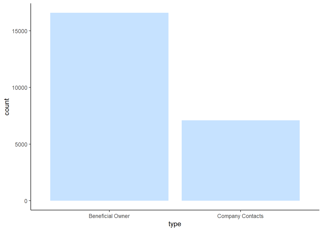
Similarly, skim() of skimr package is used to display the summary statistics of mc3_nodes tibble data frame. The report reveals that there is 21,515 missing values for revenue_omu variable.
skim(mc3_nodes)| Name | mc3_nodes |
| Number of rows | 27622 |
| Number of columns | 5 |
| _______________________ | |
| Column type frequency: | |
| character | 4 |
| numeric | 1 |
| ________________________ | |
| Group variables | None |
Variable type: character
| skim_variable | n_missing | complete_rate | min | max | empty | n_unique | whitespace |
|---|---|---|---|---|---|---|---|
| id | 0 | 1 | 6 | 64 | 0 | 22929 | 0 |
| country | 0 | 1 | 2 | 15 | 0 | 100 | 0 |
| type | 0 | 1 | 7 | 16 | 0 | 3 | 0 |
| product_services | 0 | 1 | 4 | 1737 | 0 | 3244 | 0 |
Variable type: numeric
| skim_variable | n_missing | complete_rate | mean | sd | p0 | p25 | p50 | p75 | p100 | hist |
|---|---|---|---|---|---|---|---|---|---|---|
| revenue_omu | 21515 | 0.22 | 1822155 | 18184433 | 3652.23 | 7676.36 | 16210.68 | 48327.66 | 310612303 | ▇▁▁▁▁ |
Let’s check for duplicates using the distinct function.
mc3_nodes_d <-distinct(mc3_nodes)In the code chunk below, datatable() of DT package is used to display the distinct mc3_nodes tibble data frame as an interactive table. Initially, there were 27,622 rows and it has now reduced to 25,027 rows. There were about 2,000 duplicate rows.
DT::datatable(mc3_nodes_d)Let’s plot a bar graph to show the type of nodes. As we can see from the barchart below, there are about 10,000 nodes for beneficial owners, 8,750 nodes for company, and 6,000 nodes for company contacts.
ggplot(data = mc3_nodes_d,
       aes(x = type)) +
  geom_bar(fill="slategray1") +
theme_classic() 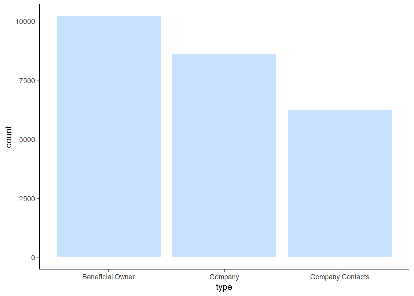
Instead of using the nodes data table extracted from the original dataset, we will prepare a new nodes data table by using the source and target fields of the aggregated edges table. This is necessary to ensure that the nodes in the nodes data tables include all the source and target values.
id1 <- edges_agg %>%
  select(source) %>%
  rename(id = source)
id2 <- edges_agg %>%
  select(target) %>%
  rename(id = target)
mc3_nodes1 <- rbind(id1, id2) %>%
  distinct() %>%
  left_join(mc3_nodes_d,
            unmatched = "drop")
We will then calculate the betweenness and closeness centrality measures.
mc3_graph <- tbl_graph(nodes = mc3_nodes1,
                       edges = edges_agg,
                       directed = FALSE) %>%
  mutate(betweenness_centrality = centrality_betweenness(),
         closeness_centrality = centrality_closeness())
Now, let’s plot the network graph using the tidygraph() function. We can see from the graph that there is a large number of nodes with high betweenness centrality, from the large circles in the middle of the graph. We will not be using this network any further, but it is interesting to see how the network is set-up!
mc3_graph %>%
  filter(betweenness_centrality >= 100000) %>%
ggraph(layout = "fr") +
  geom_edge_link(aes(alpha=0.5)) +
  geom_node_point(aes(
    size = betweenness_centrality,
    colors = "lightblue",
    alpha = 0.5)) +
  scale_size_continuous(range=c(1,10))+
  theme_graph()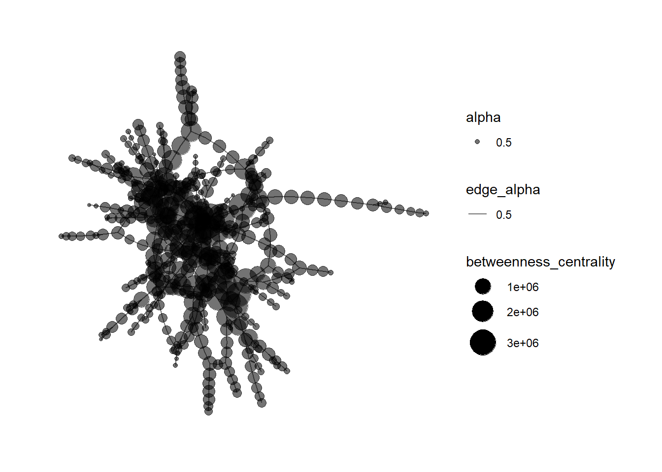
As we want to highlight possible anomalies in the dataset, we can do so by first looking at which companies have the highest revenue, and where these companies come from. To do this, let’s build a heatmap. First, we will have to join the edges_agg and mc3_nodes1 datasets so that we can create a complete dataset where there is more background information on each company.
combined_data <- left_join(edges_agg, mc3_nodes1,
                               by = c("source" = "id"))
combined_data
# A tibble: 28,852 × 8
source target type.x weight country type.y revenue_omu product_services
<chr> <chr> <chr> <int> <chr> <chr> <dbl> <chr>
1 1 AS Marine… Chris… Compa… 2 Islian… Compa… NA Scrapbook embel…
2 1 AS Marine… Debbi… Benef… 2 Islian… Compa… NA Scrapbook embel…
3 1 Ltd. Liab… Yesen… Compa… 2 Oceanus Compa… 7787. Unknown
4 1 Ltd. Liab… Angel… Benef… 2 Mawand… Compa… NA Unknown
5 1 S.A. de C… Cathe… Compa… 2 Oceanus Compa… NA Unknown
6 1 Swordfish… Danie… Compa… 2 Oceanus Compa… 6757. Unknown
7 1 and Sagl … Angel… Compa… 2 Kondan… Compa… 18529. Total logistics…
8 1 and Sagl … Chris… Benef… 2 Kondan… Compa… 18529. Total logistics…
9 2 Limited L… Amand… Benef… 2 Marebak Compa… NA Canning, proces…
10 2 Limited L… Amand… Benef… 2 Marebak Compa… NA Unknown
# ℹ 28,842 more rowsWhen we look at the dataset, we can see that there are many “unknown” and “character(0)” values under the product_services column. We should remove the rows with these values as they will not be useful for our analysis. Upon checking the results, it seems to have worked as the number of rows have now reduced from 28,852 to 10,630!
combined_data1 <- combined_data %>%
  group_by(source, target,type.x, weight, country, type.y, revenue_omu, product_services) %>%
  filter(source!=target) %>%
  rename(sourcetype = type.y) %>%
  rename(targettype = type.x) %>%
  filter(product_services != "Unknown") %>%
  filter(product_services != "character(0)") %>%
  ungroup()

#Check the dataset
combined_data1
# A tibble: 10,630 × 8
source target targettype weight country sourcetype revenue_omu
<chr> <chr> <chr> <int> <chr> <chr> <dbl>
1 1 AS Marine sanctuary Chris… Company C… 2 Islian… Company NA
2 1 AS Marine sanctuary Debbi… Beneficia… 2 Islian… Company NA
3 1 and Sagl Forwading Angel… Company C… 2 Kondan… Company 18529.
4 1 and Sagl Forwading Chris… Beneficia… 2 Kondan… Company 18529.
5 2 Limited Liability … Amand… Beneficia… 2 Marebak Company NA
6 2 Limited Liability … Megan… Company C… 2 Marebak Company NA
7 2 Limited Liability … Monic… Company C… 2 Marebak Company NA
8 2 Limited Liability … Teres… Beneficia… 2 Marebak Company NA
9 3 Limited Liability … Rober… Company C… 2 Oceanus Company 26867.
10 3 Ltd. Liability Co … Eliza… Company C… 2 Oceanus Company 112667.
# ℹ 10,620 more rows
# ℹ 1 more variable: product_services <chr>Since we are interested in knowing more about the companies, let’s select some relevant details for the dataset, such as the country, weights, revenue, and their product services. It will not be useful to look at all the companies, so let’s look at the Top 50 companies, which will be the second portion of the code chunk.
#Select the fields we want first
combined_data2 <- combined_data1 %>%
  select (source, sourcetype, country, weight, revenue_omu, product_services) %>%
  group_by(source) %>%
  arrange(desc(revenue_omu)) %>%
  distinct() %>%
  ungroup()

#Filter the top 50 companies
combined_data_top50 <- combined_data2 %>%
  filter (sourcetype == "Company") %>%
slice_max(order_by = revenue_omu, n = 50)When we look at the heatmap, we can see that the y-axis comprises of the various countries the companies are from, and the x-axis are the different companies. The different shades of blue indicate the varying revenue, from $3,652 up till $310.6million - such a wide range!
Looking at the chart, we can see that country ZH has the most number of companies which have the highest revenue (Jones LLC and Patton Ltd), which can be considered an anomaly, since no other country for the Top 50 companies have such high revenue.
#Build the heatmap
ggplot(combined_data_top50, aes(x = source, y = country, fill = revenue_omu)) +
  geom_tile() +
  labs(x = "Company", y = "Country", title = "Top 50 Companies by Revenue") +
  scale_fill_gradient(low = "lightblue", high = "darkblue") +
  theme_minimal() +
  theme(axis.text.x = element_text(angle = 90, hjust = 1))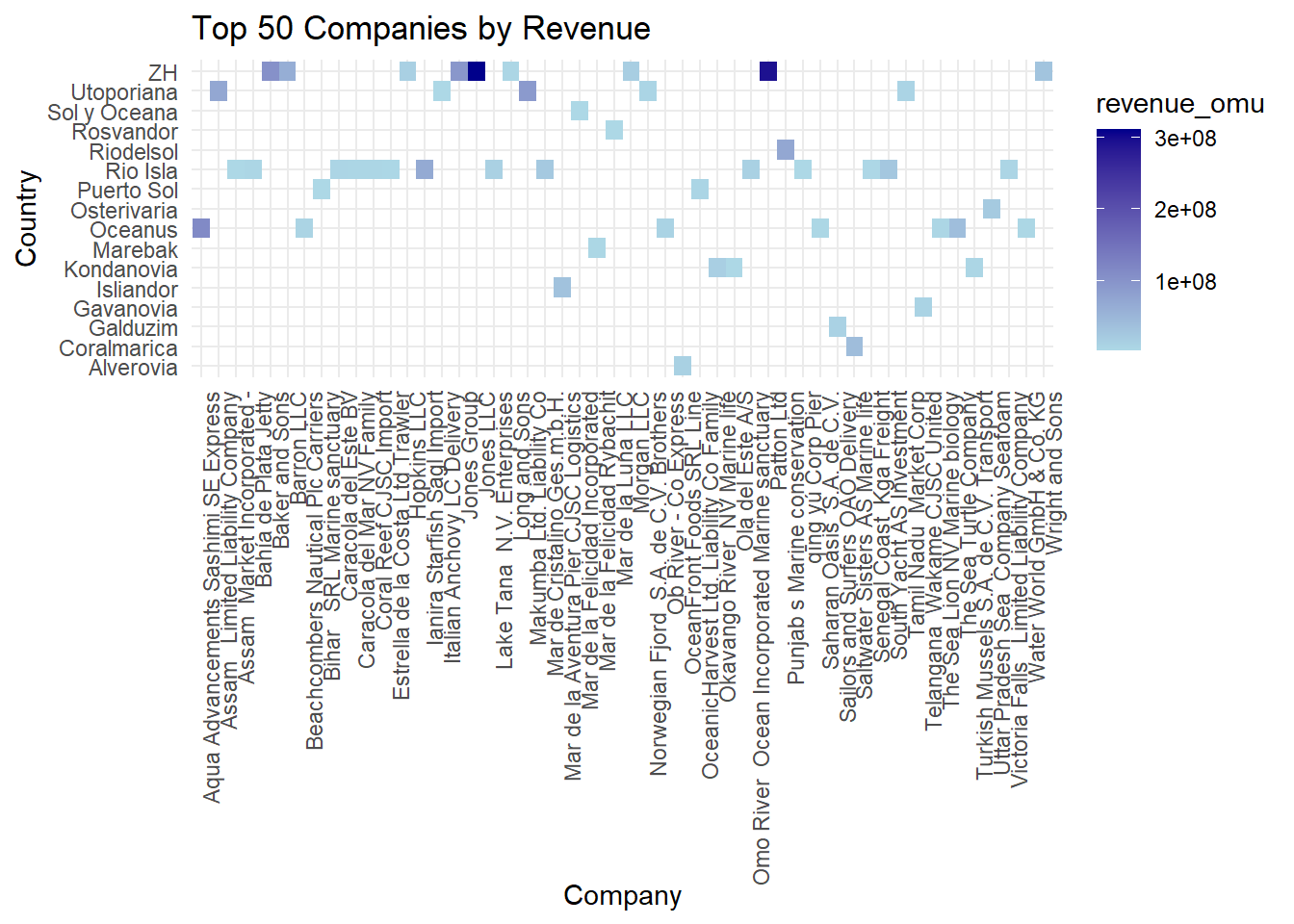
A key indicator of a red flag is actually vessel identity fraud in IUU. A vessel may use more than one identity, appearing under different names in different jurisdictions, or may use the identify of another genuine vessel, which results in 2 or more vessels having the same identify concurrently. Along the same vein, some owners may actually set up shell companies to transfer the illegal catches while concurrently conducting legitimate business under other names, and these shell companies may be set up in different countries to avoid detection.
As such, these last 2 insights will look at different ways possible anomalies may arise. Let’s look at the owners - do any owners own perhaps more than 3 companies?
For this, we would first filter out the beneficial owners, and then filter those who own more than 3 companies. However upon plotting the chart, there were more than 10 owners who had at least 4 companies, so let’s change the limit to 5 and more.
#Filter out the owners
combined_data_owners <- combined_data %>%
  select (target, source, type.x, weight) %>%
  group_by(target) %>%
  filter(type.x == "Beneficial Owner") %>%
  rename (owner = target) %>%
  rename (cmpny = source) %>%
  distinct() %>%
  ungroup()

#Filter individuals who own 5 and more companies
combined_data_owners_5 <- combined_data_owners %>%
  group_by(owner) %>%
  filter(n() > 4) %>%
  ungroup()

#Summarise count of companies per owner
companies_per_owner <- combined_data_owners_5 %>%
  group_by(owner) %>%
  summarize(Count = n()) %>%
  arrange(desc(Count))

#Check resulting dataset
companies_per_owner
# A tibble: 23 × 2
owner Count
<chr> <int>
1 John Smith 9
2 Michael Johnson 9
3 Jennifer Smith 8
4 James Smith 7
5 John Williams 7
6 Michael Williams 7
7 David Jones 6
8 Lisa Johnson 6
9 Richard Smith 6
10 Amy Williams 5
# ℹ 13 more rowsLooking at the barchart, we can see that there are 14 owners who own 5 companies, and 9 owners who own MORE THAN 5 companies. In fact, 2 of them - John Smith and Michael Johnson - own 9 companies each, and Jennifer Smith owns 8 companies. I think this is definitely an anomaly which should be taken into consideration for further investigation by the relevant authorities.
ggplot(companies_per_owner, aes(x = reorder(owner, -Count), y = Count)) +
  geom_bar(stat = "identity", fill = "slategray1") +
  labs(x = "Owner", y = "Number of Companies", title = "Number of Companies per Owner") +
  theme_classic() +
theme(axis.text.x = element_text(angle = 45, hjust = 1)) 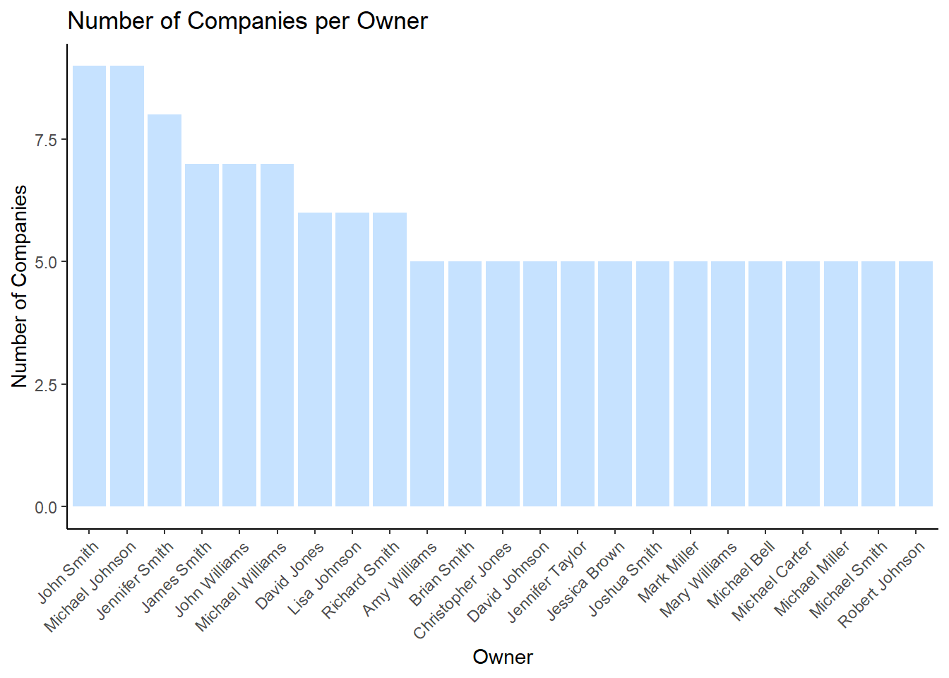
As stated above, we have highlighted 3 owners who owned than 7 companies, which is a red flag in terms of shell companies. The last red flag we would want to explore is to find out if there are any companies which are registered to more than 2 countries, as this could be a sign of company identity fraud. We keep 2 as the threshold as it’s possible that perhaps the Headquarters is in one country, and the subsidiary company is in another one.
We would first need to filter out all the companies, and then see which ones are registered in more than 2 countries. There were 53 lines of record which met the criteria.
#Filter out all companies
combined_data_countries <- combined_data %>%
  select (source, country, type.y) %>%
  group_by(source) %>%
  filter(type.y == "Company") %>%
  distinct() %>%
  ungroup()

#Filter those that are registered in more than 2 country
combined_data_countries1 <- combined_data_countries %>%
  group_by(source) %>%
  filter(n() > 2) %>%
  ungroup()

#Check dataset
combined_data_countries1
# A tibble: 53 × 3
source country type.y
<chr> <chr> <chr>
1 Aqua Aura SE Marine life Mawazam Company
2 Aqua Aura SE Marine life Rio Isla Company
3 Aqua Aura SE Marine life Icarnia Company
4 Aqua Aura SE Marine life Oceanus Company
5 Aqua Aura SE Marine life Nalakond Company
6 Aqua Aura SE Marine life Coralmarica Company
7 Aqua Aura SE Marine life Alverossia Company
8 Aqua Aura SE Marine life Isliandor Company
9 Aqua Aura SE Marine life Talandria Company
10 Bahía del Sol Corporation Novarcticaa Company
# ℹ 43 more rowsWe can see from the barchart that Aqua Aura SE Marine Life is registered in a whopping 9 companies! Next would be Transit Limited Liability Company and Tamil Nadu, which are registered in 4 countries. It would be beneficial to flag these 3 countries as an anomaly.
# Plot the bar chart
ggplot(data = combined_data_countries1, aes(x = source)) +
  geom_bar(fill = "slategray1") +
  coord_flip() +
  xlab("Companies") +
  theme_classic() +
  ylab("No of countries registered") +
  theme(axis.text.y = element_text(size = 9))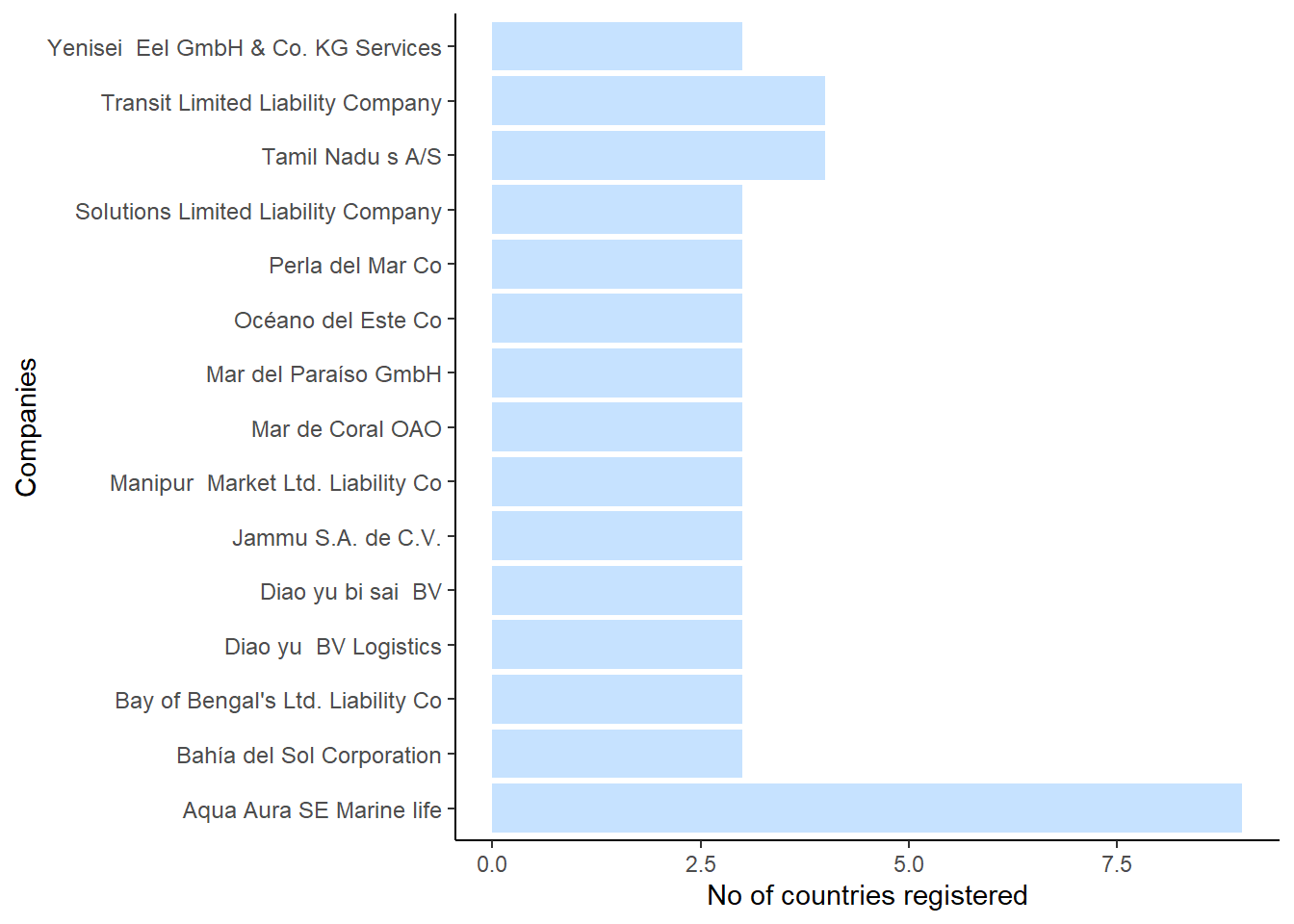
Upon knowing that Aqua Aura spans across 9 companies, I went to check its owners. Interestingly, it has more than 30 owners. Of course, beneficial owners refer to any individuals or entities that ultimately own, control, or benefit from a company or asset. Since ownership structures can be complex, the number of beneficial owners can vary depending on factors such as the size of the company, its ownership structure, and the legal requirements of the jurisdiction in which the company operates. In this case, it is possible that all of these owners are joint stakeholders. Nonetheless, it bears further investigation.
There are a few anomalies which are of concern. Firstly, there are a number of companies which are pulling in high revenue and are concentrated in country ZH. It’s possible that the conditions around ZH are ripe for IUU and thus perhaps there can be more monitoring in those seas.
There are also 3 owners who seem to own an extremely high number of companies, which may suggest the existence of shell companies which are used to launder the illegal proceeds from IUU. It would be prudent to check into the backgrounds of these individuals.
There are also a few companies which are registered to more than 2 countries. This is also a possible red flag for the shell companies and money laundering, and thus should be checked thoroughly in terms of their records to ensure that they are legitimate businesses.